Deep object detection network benchmarking and sensitivity analysis.

Introduction

Deep object detection methods represent the pinnacle of cutting edge object detection methods.

Background

Object Detection

Dealing with object in images can loosely be broken down into 4 main categories (at the time of making this post anyways). The first method of dealing with objects in images is “Object Classification”. In this task, an entire image is taken to represent a single kind of object, and the goal is to classify the image. The next, more advanced task is Object Classification with “Localization”. In this task, we try to determine two things. The first is where the object is within an image, and the second is to classify what object is in that location. The next task is “Object Detection”. This builds on Object Classification with Localization by finding multiple regions likely to have an object, then classifying each region as an individual object. The final task is “Instance Segmentation” (Image Segmentation), where the meaningful objects within an image are organized into singular segments. For our project, we focus on the “Object Detection” task. A visual representation of the different kinds of tasks is provided below.

Object Detection Tasks

As stated above, the Object Detection task is comprised of two parts. The first part deals with generating what are called “Object Proposals”. Object Proposals are regions of an image that are considered likely to contain an object. The actual object proposal task can be performed by many algorithms. These object proposals are then passed to an Object Classification algorithms that classifies each region as an object (typically with some sort of confidence). Object Proposal and Object Classification used to be considered as two seprate tasks, requiring a dedicated algorithm for each. However, more recent Object Detection methods incorporate both the Object Proposal and Object Detection tasks into a single deep neural network architecture, thus creating a single network that can perform the full end to end Object Detection.

Object Proposals and Classification

Deep Object Detection Network Sensitivity

There has been increasing interest in deep neural network based Object Detection method’s sensitivity to errors or variations in images. Currently, most of the focus is in the context of “Adverserial Attacks”, in which an image is specifically designed to trick a deep neural network into misclassifying the image with high confidence. In this scenario, some deep neural network repeatedly probes an Object Detection network with an image, iteratively modifying it to a small degree until the deep neural network misclassifies it. In some cases, the modifications that need to be made to an image to trick a deep neural network are so small that they are not visible to the human eye. This issue is visually depicted below.

Adverserial Object Detection

Another kind of deep neural network sensitivity is a deep neural network’s ability to correctly detect and classify objects in the presence of noise, or what we call “natural” image variation. We make this particular distinction from the adverserial case because these kinds of image variations are not mathematically constructed for the purpose of tricking a deep neural network. These are images that may have saturation, contrast, lighting, noise, blur, and other kinds of issues that may be naturally occuring. From our searches, we have not been able to find anyone that has previously proposed this kind of distinction for image variation. In our project, we focus on these types of “natural” image variations, and analyse the sensitivity of deep neural networks to this kind of image variation. A visual representation of some of examples of natural image variations are given below.

Natural Image Variation Object Detection

Project Proposal

Problem?

For this project, we focused on 3 main questions related to deep neural network based object detection methods.

1. How sensitive are cutting edge deep object detection networks to natural noise/errors/variation in images?

2. What kind of process and metrics should be used to quantify this sensitivity?

3. Can our analysis be used to provide a context of which networks to use in different contexts?

Importance?

1. Safety Applications: A practical understanding or methodology for determining how Deepnets fail is crucial if we expect to use deep nets in safety concerned applications, such as autonomous driving.

2. Context Specific Applications: Field focus is on “new” networks. Little knowledge of practical use “in the wild”.

3. Lack of Rich Performance Metrics: Standard ML metrics don’t map very well to object detection. There aren’t rich metrics that quantify things like “color sensitivity”

State of the art?

We aim to benchmark some of the most commonly used, modern deep neural networks including Mask R-CNN , RetinaNet , Faster R-CNN , RPN , Fast R-CNN , and R-FCN . Some of the pre-trained backbone networks we are looking to use include ResNeXt{50,101,152} , ResNet{50,101,152} , Feature Pyramid Networks , and VGG16 . The datasets we aim to use include the COCO dataset, PASCAL VOC dataset, and the Kitti object detection dataset. These network architecture designs, and network backbones represent some of the most common cutting edge object detection deep neural networks that exist today.

In terms of actual analysis, not much work has been performed into analysis of deep neural network models other than basic average performance metrics of individual models. Most work focuses more on proposing a new architecture for a deep network object detection model, rather than comparing its significant difference with existing methods, major fundamental drawbacks, and other ways in which the network can be fooled or broken. We provide a general summary of some of the state of the art networks, backbones, data sets, and kinds of analysis.

• Networks:
  • Mask R-CNN, RetinaNet, Faster R-CNN , RPN , Fast R-CNN , R-FCN, YOLO
• Backbones:
  • ResNeXt{50,101,152} , ResNet{50,101,152} , Feature Pyramid Networks , and VGG16
• Datasets:
  • COCO (Multi-object Detection Dataset)
  • PASCAL VOC (Multi-object Detection Dataset))
  • Kitti (Autonomous Vehicle Object Detection Dataset)
• Analysis:
  • Simple aggregated performance metrics
  • Adversarial based analysis

Existing Systems or New Approach?

We plan on benchmarking existing neural network designs and implementations that are representative of current deep neural network object detection based methods, with one particular goal being a proposal and outline of future research work that should be developed to address some of the issues we find. This might fall under the category of a “new approach”. However, we also plan on performing deeper analysis of existing methods than has been previously performed to provide for a better overall understanding of how well modern methods compare, how similar and different the methods are, which approaches seem to work the best, and what shortcoming exist with existing methods.

Evaluation and Results Plan?

Our project proposal centers around benchmarking and analyzing different deep object detection networks, so the evaluation phase is really the meat of our project (aside from getting everything up and running). The details of what we plan on benchmarking, what platforms we plan to use, what data sets we plan to use, and what metrics we plan to calculate are given in the “Approach” section below.

Approach

High Level Steps

1. Select the most cutting edge object detection networks.
2. Perform performance analysis on a base set of images for each network.
3. Generate images with “natural” errors/noise/artifacts/transforms.
4. Perform performance analysis on transformed images for each network.
5. Compile sets of summary metrics organized by object classes, transform kind, and model.
6. Compare and contrast performance to draw insights about deep network capabilities and sensitivities based on class, transform kind, and model.
7. Create guidelines for developing and using deep object detection networks, and propose new data.

Networks, Images, Datasets

Below, we outline the networks we tested, the analysis we performed, and the systems we used.

• 10 Networks (Requires 11GB Graphics Cards):

  • <Net Arch>_<Net Backbone>-<Proposals>_2x
  • e2e_faster_rcnn_R-101-FPN_2x
  • e2e_faster_rcnn_R-50-C4_2x
  • e2e_faster_rcnn_R-50-FPN_2x
  • e2e_faster_rcnn_X-101-64x4d-FPN_2x
  • e2e_mask_rcnn_R-101-FPN_2x
  • e2e_mask_rcnn_R-50-C4_2x
  • e2e_mask_rcnn_R-50-FPN_2x
  • retinanet_R-101-FPN_2x
  • retinanet_R-50-FPN_2x
  • retinanet_X-101-64x4d-FPN_2x

• Images:

  • COCO image validation data set.
  • 5000 base images (600x800 3 channel images)
  • 50 Transforms generating 250,000 images total
  • 5000*5010(300 proposals/net) = 750 Million object candidates

• Systems:

  • 8 GTX 1080ti GPU system with 11GB per Card, 8 GB Ram
  • i7 CPU, 24GB Ram
  • University of Wisconsin Condor GPU Instances

Image Transforms

We have 50 image transforms that we applied to the COCO validation image set. There are roughly two categories of image transforms that we applied. The first is value based transforms. Most of these transforms deal with changing images in ways related to the value of pixels in an image. The second is spatial based transforms, in which we transform images in ways that may alter the phisicaly size, shape, or arraingment of pixels within an image. We provide some visual examples of each kind of image transform below.

Value Based Transforms

Spatially Based Transforms

Set of All Transforms

transformNames = [ ‘None’, ‘gaussianblur_1’, ‘gaussianblur_10’, ‘gaussianblur_20’, ‘superpixels_0p1’, ‘superpixels_0p5’, ‘superpixels_0p85’, ‘colorspace_25’, ‘colorspace_50’, ‘averageblur_5_11’, ‘medianblur_1’, ‘sharpen_0’, ‘sharpen_1’, ‘sharpen2’, ‘addintensity-80’, ‘addintensity_80’, ‘elementrandomintensity_1’, ‘multiplyintensity_0p25’, ‘multiplyintensity_2’, ‘contrastnormalization_0’, ‘contrastnormalization_1’, ‘contrastnormalization_2’, ‘elastic_1’, ‘scaled_1p25’, ‘scaled_0p75’, ‘scaled0p5’, ‘scaled(1p25, 1p0)‘, ‘scaled(0p75, 1p0)‘, ‘scaled(1p0, 1p25)‘, ‘scaled(1p0, 0p75)‘, ‘translate(0p1, 0p1)‘, ‘translate(0p1, -0p1)‘, ‘translate(-0p1, 0p1)‘, ‘translate(-0p1, -0p1)‘, ‘translate(0p1, 0)‘, ‘translate(-0p1, 0)‘, ‘translate(0, 0p1)‘, ‘translate_(0, -0p1)‘, ‘rotated_3’, ‘rotated_5’, ‘rotated_10’, ‘rotated_45’, ‘rotated_60’, ‘rotated_90’, ‘flipH’, ‘flipV’, ‘dropout’, ]

System

Systems Overview

Our system processing pipeline consits of a general processing scheme of CPU->GPU->CPU. We perform initial image transfromations on our CPU based system. Then, these images are shipped to a GPU based cluster and other GPU based systems to perform inference. During inference, a set of json object output files are generated containing the predicted bounding boxes, classes, and confidence scores over every image. These output files are then sent back to our CPU based system where we convert bounding boxes and confidence scores to hard predictions. Once the hard predictions of objects has been made, we use some parallelized CPU based scripts to generate precision and recall values over all combinations of models, transforms, and class (10 models * 50 transforms * 88 classes). We then analyze these results in an .ipynb, which can be seen below in the results section.

Results

In this section we detail the results of our analysis. Below, we show and describe some of the main plots we created during our analysis. However, many of the tables are descriptive examples of our analysis are cut down. The full set of results from the IPython notebook can be viewed at the link below. We discuss the metrics we currently use for performane analysis, and discuss some of the plots we generate, and how they can be used to gain further insight into the performance of particular combinations of model type, image tranform type, and class category.

IPython Notebook Analysis Results

Current Metrics

Currently, we rely on straight Precision and Recall based metrics to perform analysis. We’ve found that most papers produce either precision only metrics, or metrics such as unweighted mean average precision, which favor high precision and low recall models (which is somewhat stated in the PASCAL paper and the original Information Retrieval paper for which mean average precision is based on). We’ve also noticed that for many papers, the numbers presented tend to be only for “favorable” class categories, and aren’t given the proper context considering class skew and P/R curve distributions. For the most part, we’ve found that the results shown in papers are not good indications of actual network performance, and that the metrics used are more useful for discriminating between “rough average performances” over sets of tasks, and should not be used for determining network performance on a specific task.

• Precision and Recall
  • Precision: How confident are we when the model predicts a dog, that the object is a dog, and not something else?
  • Recall: How many of the instances within a class are actually found?
• Combinations
  • For each combination of “Model, Image Transform Type, Class Category”, we generate a single precision and recall value. We then use OLAP style analysis over these values to aggregate and average performance metrics to get better insight.

Precision Recall Histograms

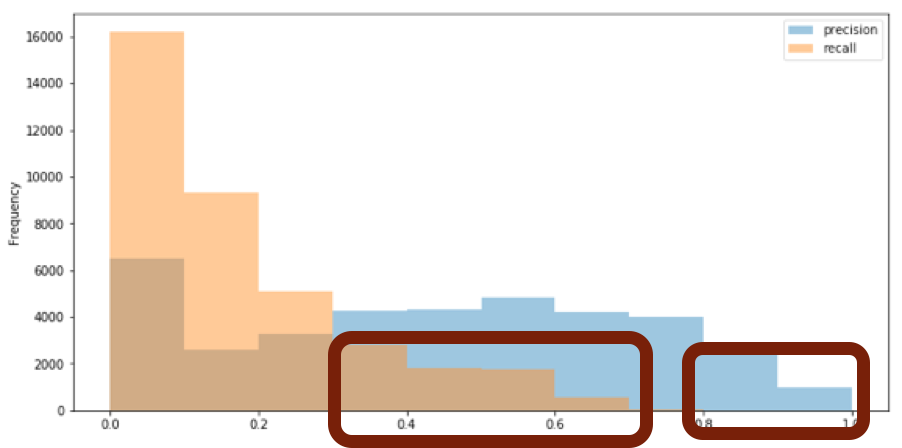
The histograms below represent the precision and recall metrics for all model, transform, and class combinations. More specifically, say for the combination of model e2e_faster_rcnn_R-50-C4_2x, a transform of ‘gaussianblur_1’, and class label ‘person’, we measured a precision of 0.714 and a recall of 0.277 (Given an Intersection over Union of 0.5). For each of the potential combinations, we generated a precision and recall, and plotted all of the measures as histograms. We did this to give us a general idea of the overall performance of the deep object detection networks. Our average precision was around 0.53, and for some classes was much higher. However, for most classes, recall was 0.25 or below (for some it was higher, but this was due to class skew and not reliable performance). The red squares below highlight the issues of combinations that had either high precision, or high recall, but most of these combinations were due to class skew. As we discuss later on, there tends to be a trend of high precision, low recall models for the COCO object detection data set that tends to be obscured by the traditional mean average precision metrics that are used to evaluate models. We talk more about these issues later.

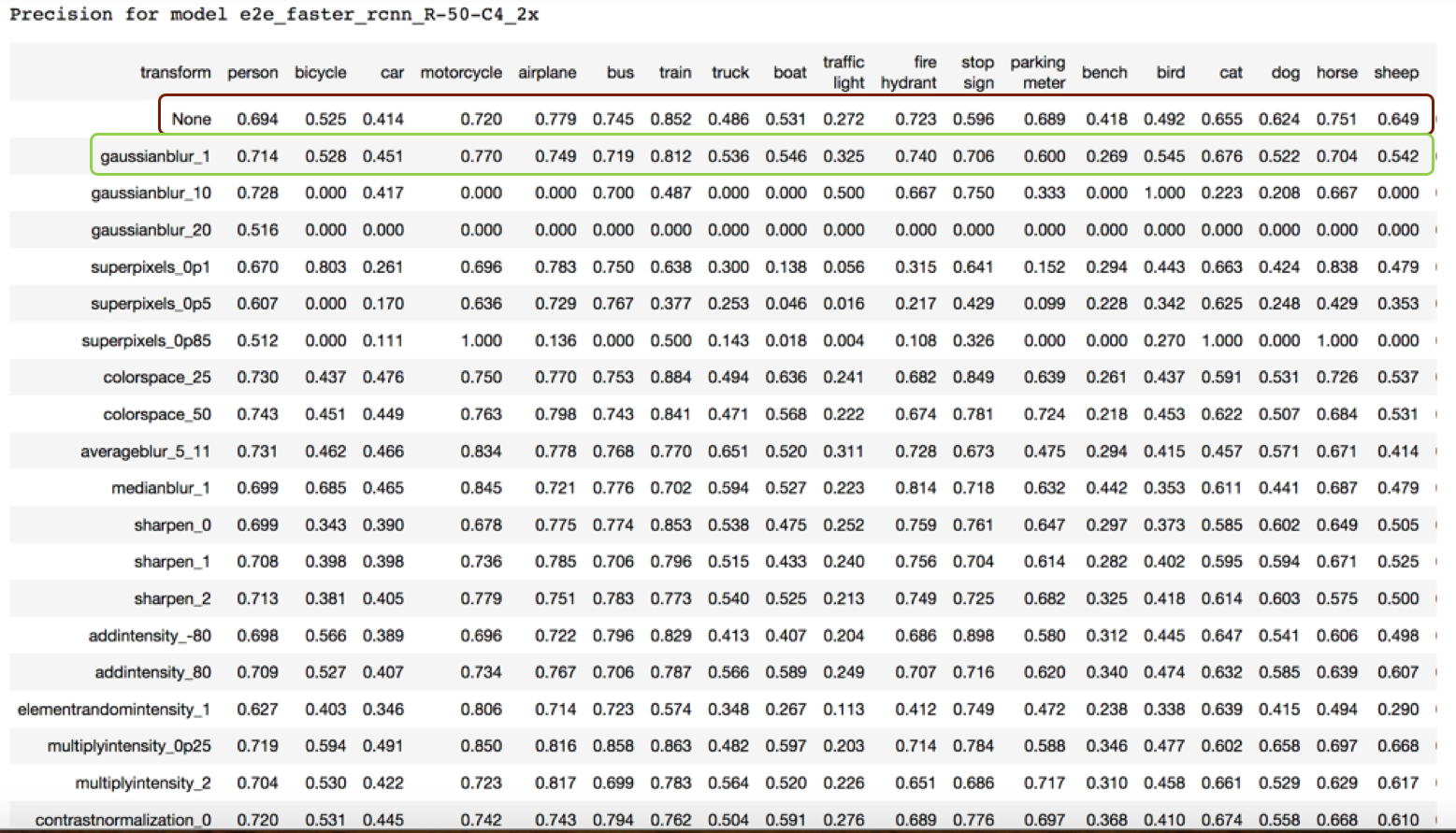
Precision per (model,transform,class)

The table below shows a slice of a table describing precision for a specific model (in this case, the model is “e2e_faster_rcnn_R-50-C4_2x”). The columns of the table relate to a specific class (except the first column), and each row corresponds to a specific transform over the original data set (with the first row “None” being the original image set). For example, the first precision entry in the table 0.694 means that for the e2e_faster_rcnn_R-50-C4_2x model, on the original image set, for the person class was 0.694.

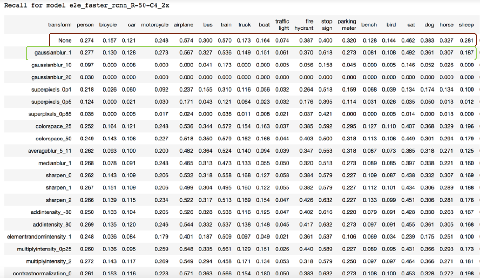
Recall per (model,transform,class)

The table below shows a slice of a table describing recall for a specific model (in this case, the model is “e2e_faster_rcnn_R-50-C4_2x”). The columns of the table relate to a specific class (except the first column), and each row corresponds to a specific transform over the original data set (with the first row “None” being the original image set). For example, the first recall entry in the table 0.274 means that for the e2e_faster_rcnn_R-50-C4_2x model, on the original image set, for the person class was 0.274.

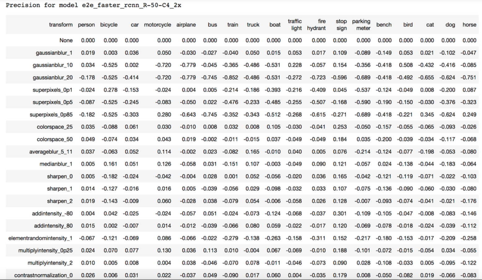
Precision difference per (model,transform,class)

The table below shows a slice of a table describing the difference in model precision between the original image set, and a specific transformed version of the original image set. A positive value indicates a performance increase, and a negative value indicates a performance decrease.

Precision per (class,transform) avg over model

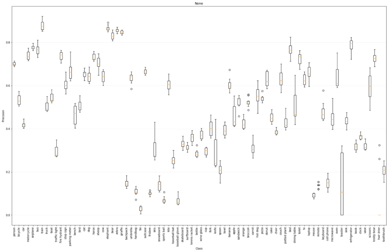
Each box plot below corresponds to a single transform, and shows the average precision over all models on a per class basis. The plot below shows the averaged precision over all models on the original data set.

The plot below shows the averaged precision over all models on the gaussian transform data set with a sigma of 1.

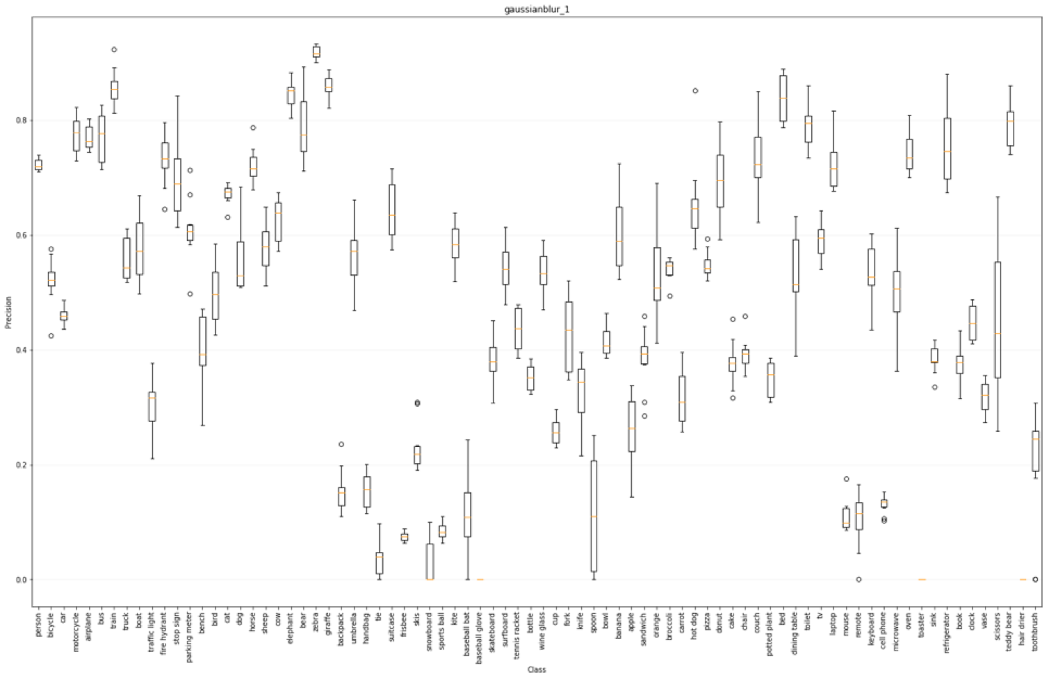
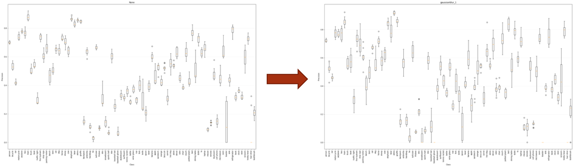
The key usefulness of these plots is to compare how each transform affects the aggregated performance over all models on a per class basis, or in general. For example, the left plot below corresponds to the original data set, and the right plot corresponds to the gaussian blurred data set. As you can see, for some classes, precision increased, and for other classes, the precision decreased.

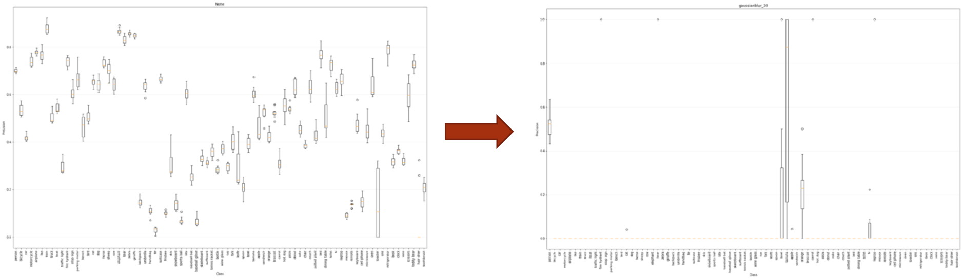
In the plot below, the left plot corresponds to the original data set, and the right plot corresponds to the gaussian blurred data set with a sigma of 20. As can be seen from the plot, performance is severely degraded when a large amount of gaussian blur is added to an image.

Precision per (model) avg over transform and class

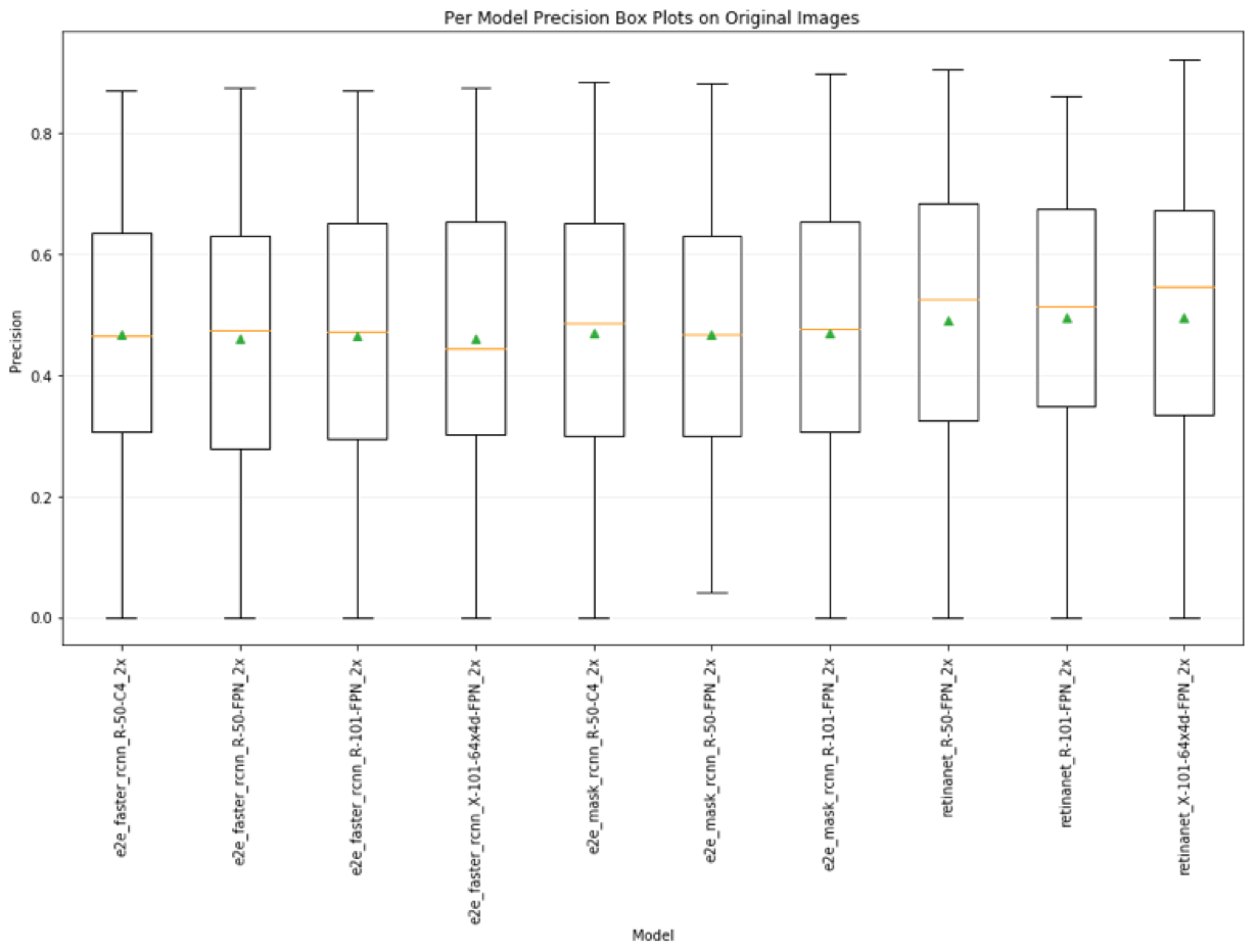
The plot below shows a box plot for precision for each model, averaged over all transformed image sets and classes. The yellow bar is the median performance, and the green triangle is the average performance. On average, the precision for the retina net 101-64x4d-FPN model performs better than the other models. However, we can’t conclude anything about raw specific performance since the confidence bounds of every set of models is nearly the same.

Recall per (model) avg over transform and class

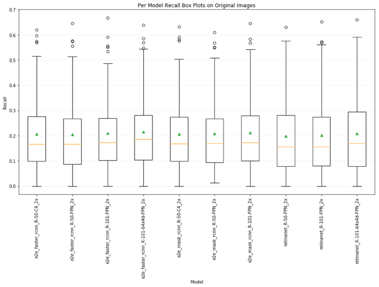
The plot below shows a box plot for recall for each model, averaged over all transformed image sets and classes. The yellow bar is the median performance, and the green triangle is the average performance. On average, the recall for the faster rcnn 101-64x4d-FPN model performs better than the other models. However, we can’t conclude anything about raw specific performance since the confidence bounds of every set of models is nearly the same. We can see that recall is very low across all models. While there are some models with high recall (which doesn’t tell us much since we don’t also see their corresponding recall), these cases are clearly outside of the confidence bounds for the performance over all model.

Average precision difference given each transform category

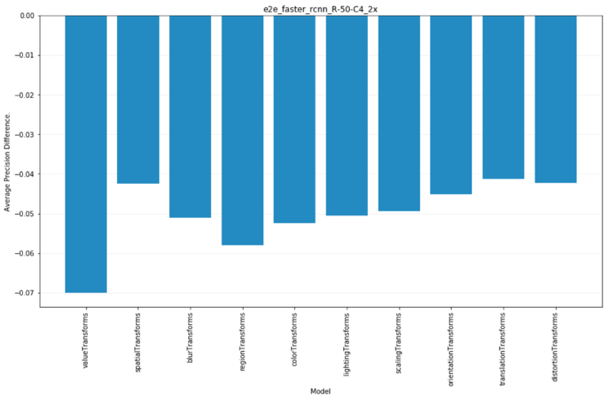
Each plot below corresponds to a single model. The bars correspond to the average precision difference for the model between the original image set, and all image sets in the specified “category” or transform, over all classes. The first two bars show the highest categories of value based transforms and spatial based transforms. As can be seen from the plot, value based variations in images affect model performance on average more than spatially based transforms. The rest of the bars show the average precision difference over other categories of transforms. The set of all plots, as with the other plots shown in this section, can be viewed from the link to the full analysis outputs link at the beginning of this section. The set of all categories is given below.

• valueTransforms = [blurTransforms, regionTransforms, colorTransforms, lightingTransforms]
• spatialTransforms = [scalingTransforms, orientationTransforms, translationTransforms, distortionTransforms]
• blurTransforms = [ ‘gaussianblur_1’, ‘gaussianblur_10’, ‘gaussianblur_20’, ‘averageblur_5_11’, ‘medianblur_1’]
• regionTransforms = [ ‘superpixels_0p1’, ‘superpixels_0p5’, ‘superpixels_0p85’, ‘averageblur_5_11’]
• colorTransforms = [‘colorspace_25’, ‘colorspace_50’, ‘multiplyintensity_0p25’, ‘multiplyintensity_2’, ‘contrastnormalization_0’, ‘contrastnormalization_1’, ‘contrastnormalization_2’]
• lightingTransforms = [‘sharpen_0’, ‘sharpen_1’, ‘sharpen2’, ‘addintensity-80’, ‘addintensity_80’, ‘elementrandomintensity_1’]
• scalingTransforms = [ ‘scaled_1p25’, ‘scaled_0p75’, ‘scaled0p5’, ‘scaled(1p25, 1p0)‘, ‘scaled(0p75, 1p0)‘, ‘scaled(1p0, 1p25)‘, ‘scaled_(1p0, 0p75)‘]
• orientationTransforms = [ ‘rotated_3’, ‘rotated_5’, ‘rotated_10’, ‘rotated_45’, ‘rotated_60’, ‘rotated_90’, ‘flipH’, ‘flipV’]
• translationTransforms = [‘translate(0p1, 0p1)‘, ‘translate(0p1, -0p1)‘, ‘translate(-0p1, 0p1)‘, ‘translate(-0p1, -0p1)‘, ‘translate(0p1, 0)‘, ‘translate(-0p1, 0)‘, ‘translate(0, 0p1)‘, ‘translate(0, -0p1)‘]
• distortionTransforms = [‘elastic_1’, ‘dropout’]

Discussion

Short Summary

Long Summary

Issues

1) Most networks are super brittle and need more work to make them robust.

• Any image variation impacts performance.
• Significant sensitivity to training image set.

2) Most evaluation metrics are average metrics.

• Weighted average is disingenuous for performance across multiple classes.
• There should be a diminishing marginal benefit performance metric.
• Precision only (which most papers report) covers up low recall.
• Recall IoU, only shows recall profile, not coupled recall and precision.
• The way in which multi-class P/R averages are generated is not well specified.

Real World Guide

1) Blur

• Well defined boundary objects (cars, trains, bus, bench, etc…) small blur is bad
• Less well defined boundary objects, or moving objects with more variety (people, dogs, birds, etc…) small blur tends to be good.

2) Image size

• Applications with large objects are better. In fact, if dealing with small objects, artificially scale image size to increase network performance.

3) Add contrast to your images.

• Networks are very sensitive to the magnitude of relative intensity differences in images. Amplify these differences for improved performance.

4) Locality based jitter and noise is really bad.

• Severely decreases performance. (Brownian motion type deal)

5) Center objects in images.

• More centered objects are detected more often and more precisely than objects near edges.

6) Region textures matter in an object.

• Superpixel transforms show degraded performance for larger contiguous regions with same color and no textures.

7) Hues and alternate color spaces

• Adjusting hue values up increased performance on average. (Color contrasting affects)

Project Next Steps

Next Steps for This Project?

Sensitivity Analysis Toolkit.

In our extensive literature review, we have not found any major initiatives or projects that are focused on analyzing and quantifying the sensetivity of an object detection network to natural variation in images. We believe that there would be value in working towards trying to create a toolkit for testing and measuring object detection sensetivity for both research and practical applications.

New Sensitivity Metrics.

Another thing that we’ve noticed in our literature review was that many of the performance metrics that are used for measuring deep object detection networks come from traditional machine learning and information retrieval areas. However, rich performance metrics related to the image object detection context are lacking. Sensitivity metrics, like the ones we’ve showed above related to kinds of variation are benneficial. Other rich metrics could also be feasibly constructed such as objectness variability for specific classes. New sensitivity metrics such as these would provide better insight for developing and applying deep object detection networks, which is currently ambiguous and undirected.

Next Steps for This Area?

• Amount of re-training needed to reduce errors?
• Architectural changes/constraints needed to reduce errors?
• How much reducing network size for memory/speed affects errors?

Notes Code on Github 4 days to run on our hardware (parallelize by 8) 4*8=32 days to run on single GPU single core system

Special Thanks

Special thanks to Matt Nichols for providing us access to his 8 GPU bitcoin mining machine! Without access to such a powerful system, this project would not have been possible.

Appendix

Challenges We Faced

Refactoring our project and proposal.

• So we had to rapidly change our direction when we realized the tedious complexity of our original project proposal, and search for a new potential project. We had to review lots of object detection papers and methods to come up with a new project to work on. Once we had an idea that we wanted to try to perform a set of benchmarking, we had to find candidate models, platforms, frameworks, datasets, and metrics that we thought we could achieveably use for our project. Some of the challenges of these are found in the next subsections.

Running on Condor GPUs and getting access to resources.

• Most of today’s existing deep neural network, object detection based models require GPUs (A major drawback which I believe will eventually be remedied with FPGAs due to their high speed, low power nature which makes them a defacto choice for most industry scale, long term use). So, we talked to the University of Wisconsin’s HPC group about running on the GPU based condor instances. We spent a good amount of time writing the submission and monitoring scripts for the GPU instances, and in particular the docker based GPU instances to simplify code submission. However, there are only 2 machines in HPC with 4 total GPUs that currently run docker, and the queue is so congested that using condor for our project became clearly impractical (I submitted a GPU based docker job about a week ago that still hasn’t been run yet). I’ve talked with the condor HPC Team Members - Daniel Griffin, Yudhister Satija staff, and they are working on getting docker running on the other 2 older instances (each with 6-8 GPUs each) that don’t have Docker (But we can’t use these without docker, as the nature of the code we are trying to run on the machines requires installation and system configuration permissions).

Running on AWS, and the cost associated with it.

• Since we couldn’t run on the condor instances, we decided to turn to Amazon Web Services (AWS) to try to provision instances. After a few days of working with AWS EC2 instances, we finally developed a process for provisioning AWS GPU instance resources for running our nvidia-docker based code, and running some of our initial deep net object detection models (Many of which need GPUs for their operators, and up to 15GB of dedicated system memory). The downside with this is that AWS GPU instances are $1/HR to provision and use which is quite expensive for compute resources (And why we are trying to avoid training models that can each take anywhere from hours to days to train).

Dataset non-uniformity.

• While there exist some different datasets for benchmarking object detection, most data sets have different formats. We have decided to try to standardize to the COCO dataset API, and to try to convert some of the other data sets we would like to use to the COCO annotation specifications. This means that we will likely have to write scripts for generating COCO annotated images from each data set.

Initial Proposal and Midterm Reports.

• Initial Project Proposal
• Midterm Report
• Project Presentation
• Github Repository

• Share this article: